Training a Protein Model From Scratch

Inspired by the numerous “GPT-2 from scratch” posts from 2 years ago, I decided to try my hand at doing the same for generative protein biology. The specific architecture I wanted to replicate was RFDiffusion, which was published in 2022.

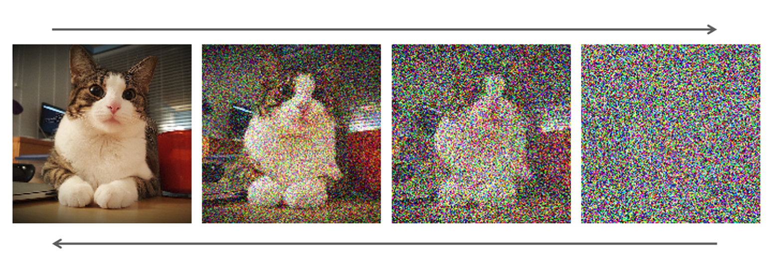
Unlike “Protein Language Models” (like ESM) which are trained on text sequences, RFDiffusion is a Structure Diffusion Model. Simplistically, it learns to denoise 3D coordinates to “dream up” brand new protein backbones that maintain the physical and chemical properties of real proteins. RFDiffusion is much closer to an image generation model like Stable Diffusion than GPT-2.

My goal was to build and train a minimal version of RFDiffusion from scratch. The code can be found here.

The Plan

At a high level, the project was broken into 4 parts.

1. Data: What dataset should I train on? How do I clean it and represent it?
2. Model: What architecture should I use? What exactly is the learning objective and loss function?
3. Training: What hyperparameters do I use for training? How much compute do I actually need?
4. Evaluation: How do I tell whether generations are “protein-like” versus garbage?

Data

While RFDiffusion was trained on Protein Data Bank (PDB), I opted to train my model on a smaller, cleaner dataset called the CATH (Ingraham split). The full PDB dataset has something in the order of ~250k structures, whereas the CATH dataset has been trimmed to ~20k structures, but they are more diverse and deduplicated. The dataset has also been cleaned up such that each protein is a single chain, whereas many of the PDB proteins are multiple chains stuck together. Each row in the dataset looks something like this:

{
  "name": "132l.A",
  "seq": "KVFGRCELAA...GCRL",
  "coords": {
    "N": [
      [-9.887, 16.726, 47.556],
      [-7.500, 18.200, 49.100],
      ...
    ],
    "CA": [
      [-8.887, 17.726, 48.556],
      [-6.200, 18.500, 49.800],
      ...
    ],
    "C": [
      [-7.527, 17.300, 48.900],
      [-5.500, 19.800, 49.200],
      ...
    ],
    "O": [
      [-7.100, 16.200, 48.700],
      [-5.800, 20.900, 49.600],
      ...
    ]
  }
}

We can see that each backbone has 4 elements (N, C, CA, O), and the dataset contains the coordinates of each one in 3D space. Instead of training the model to predict structures of all 4 elements, we can just train it on Ca atoms. This is because if we know the position of all the Ca atoms, we can algorithmically “fill in” the rest of the atoms with high confidence. We also know that Ca atoms have a fixed distance of ~3.8 Å between them, which we can later use for evaluation. This narrows down the scope of complexity of the task by quite a bit.

Model

RFDiffusion is a diffusion transformer model. It uses diffusion as the framework, where the model learns to denoise, and a transformer as the architecture for how the model learns. Instead of training from scratch, RFDiffusion actually uses RosettaFold, which is an AlphaFold equivalent model, as the base model then fine-tunes this denoisining capability on top. This lets RFDiffusion inherit the base knowledge of protein folding physics from RosettaFold. However, given that I wanted to make a mini RFDiffusion-style model, I opted to just train it from scratch instead of finetuning a protein folding model.

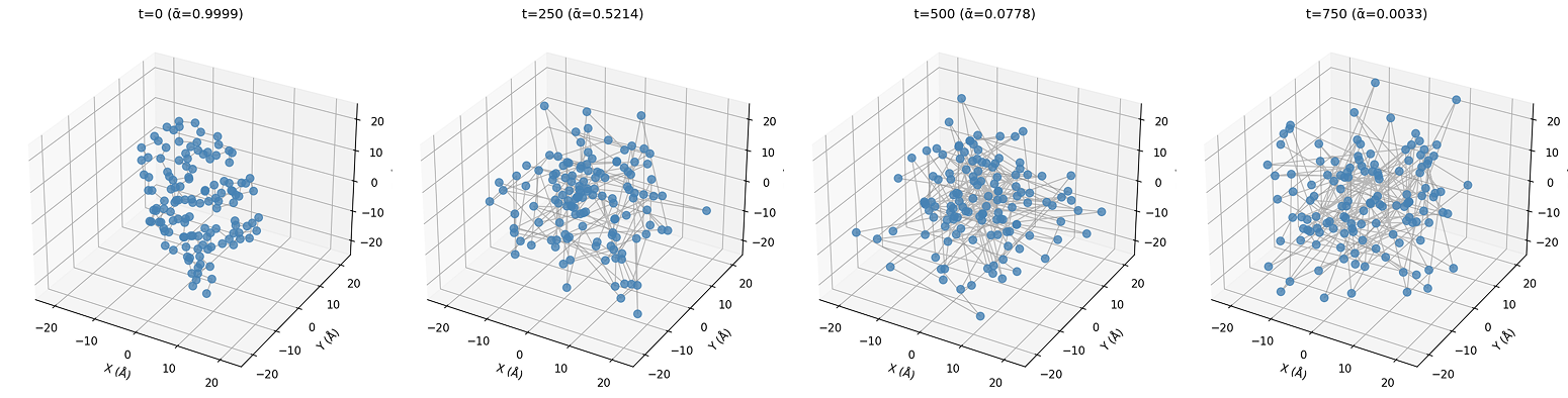
The training process looks like the following:

1. Take the coordinates of the Ca atoms from a real protein in the dataset ($X_0$)
2. Apply some noise ($t$) to it, so the coordinates are now $X_t$
3. Ask the model to look at $X_t$ and predict the noise ($\epsilon$) that was added
4. We subtract the predicted noise ($\epsilon$) from $X_t$, and effectively get $X_{0\_pred}$
5. Calculate the MSE between $X_{0\_pred}$ and $X_0$, and backpropagate that loss

The diffusion process is very similar to regular diffusion in image models.

In a text model (LLM), the attention mechanism primarily looks for semantic relationships between words, using “Positional Encodings” to understand which words are important to each other. However, proteins are folded objects. Two residues might be very far apart in the sequence (like “Q” at position 1 and “B” at position 50) but effectively touching in 3D space. If we used a standard Transformer, the model would think Residue 1 and Residue 50 are unrelated. We can modify the attention mechanism to inject a “bias” based on the actual 3D distance between atoms, forcing the model to pay attention to physical neighbors, not just sequence neighbors. This technique is called Geometric Attention.

Since we also know that Ca atoms have a fixed distance of ~3.8 Å between them, I modified the loss function to add in a penalty for generations which have atoms that drift away from 3.8. Interestingly, I found that models that had this extra penalty in the loss function were worse than the models that had to “learn” this 3.8 Å distance on its own.

Training

Training was fairly straightforward. I started with overfitting my model on a single chain to check if the model could actually learn to reproduce this structure. Then I moved to train on larger and larger chunks of the CATH dataset.

I also implemented two techniques to make the training data more robust. First, I used sliding windows, so I could get multiple data points from a single protein structure i[0:64], i[65:128]. Secondly, I applied random rotations so that the model could learn to generalize better.

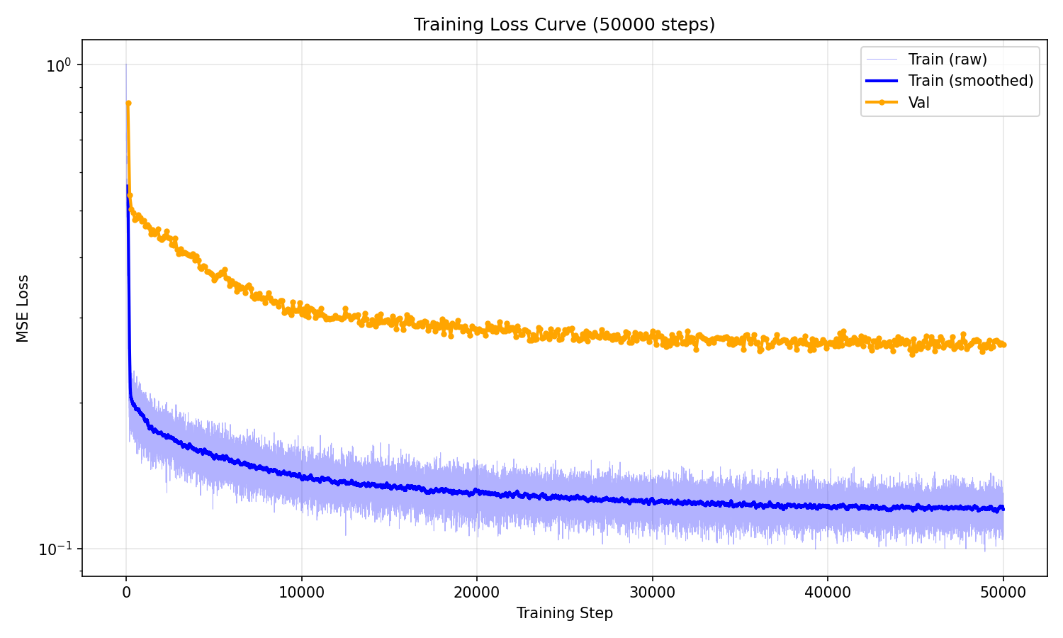
I trained the model for 50k steps on a single RTX 5090 and each run took approximately ~5 hours to complete.

Evaluation

To evaluate these models, I measured a few things:

1. Bond Length Mean: We know that bonds should be ~3.8 Å. What was the average distance between consecutive Ca atoms?
2. Valid Bond %: What percentage of bonds fell within the physically valid range (3.6 - 4.0 Å)?
3. Radius of Gyration (Rg): How “compact” was the generation? Proteins are globular; high Rg indicates the model generated “spaghetti.”
4. Clash Count: How many “clashes” (bonds which are <3.0 Å) are there?
5. Reconstruction RMSD: If we take a real protein, add noise (diffuse it), and ask the model to repair it, how close is the result to the original?

After multiple runs with various hyperparameters, here’s what ChatGPT said about the results from my best run.

Metric	Expectation	Result	Verdict
Bond Length (Mean)	~3.80 Å	3.99 Å	✅ Excellent. Slightly relaxed, but physically accurate.
Valid Bonds (%)	> 90%	96.7%	✅ Perfect. The model learned the geometry constraint.
Clashes	0.0	0.0	✅ Perfect. No self-intersections.
Radius of Gyration	~15 - 25 Å (Compact)	20.04 Å	✅ Compact. The proteins are folded, not spaghetti.
Reconstruction RMSD	< 5.0 Å	3.81 Å	✅ Success. It can recover structures from noise.

The model seems to be able to create realistic-seeming protein backbones now.

Testing

To do more realistic evaluation beyond just heuristics like bond length, I wanted to see some examples of structures that my model created, and if those would actually fold. Here’s an example of one of the samples that the model generated.

Then, I used a different model ProteinMPNN to go from backbone -> sequence, and it produced this sequence LGTLAAALAAAAA.... Lastly, I passed that sequence into AlphaFold to see what the final protein would look like.

This looks surprisingly decent for a model that was trained on a single GPU in 5 hours. However, AlphaFold’s confidence score for this protein was 0.29 pTM, which is abysmal and implies that the sequence itself would likely not fold in real life.

Generating Useful Binders

Right now, the model is basically a denoiser — given a random amount of noise, the model can predict the noise and create a structure that respects some of the physical properties of protein backbones. However, how is this actually used in practice to generate binders?

Creating a binder is very similar to the concept of inpainting in image generation models. The user provides a picture of a living room, and creates a mask around the sofa and prompts the model with a cat – then the model generates a cat that fits into the context / background of the rest of the image. We do the same thing here to generate a binder.

Here’s how it works:

• Say we have a target, ABCD, and we want to design a 2-residue binder to this target
• First, we come up with a random 2-residue sequence like XX. Now our whole structure is ABCDXX
• Setup (t=1000)
  • ABCD_1000,XX_1000
• The Loop (t=1000 -> 999)
  • Model looks at ABCD_1000,XX_1000 and predicts the noise.
  • Result = ABCD_999_pred,XX_999_pred.
  • Now we replace ABDC_999_pred with the actual ABCD_999
  • Result = ABCD_999,XX_999_pred
• Through this, you “force” the target to stay in place while you iterate through 1000 rounds of predictions.

This lets us generate structures that fit “around” the actual target that we care about, and if the structure folds with high confidence, this could be a feasible drug candidate. For example, this protein (the small green one) LCB1 was designed to attach to the COVID virus spike protein (orange), and effectively block it from interacting in the body. Generative models like RFDiffusion or others can create something like this zero-shot, whereas the original LCB1 took months of computation.

Conclusion

Given that I trained this toy model with a tiny amount of compute, I was still positively surprised by the results, and that it could even create reasonable looking structures! It makes sense that RFDiffusion was fine-tuned on RosettaFold, since that was pretrained on the entire Protein Data Bank for months and already inherits many of the fundamental physics of protein folding.

An extension project for this would be to retrain minirf on a strong protein folding model like AlphaFold3, and seeing if that creates better results than RFDiffusion.